Complexity
Last translate with upstream: a032fb3
Time complexity and space complexity are important criteria to measure the efficiency of an algorithm.
Count of Elementary Operations
An algorithm has different performances on different computers. It is hard to calculate the actual performance theoretically and is troublesome to measure it. Thus, it's more often for us to consider the count of elementary operations required by an algorithm rather than the actual time used.
For a typical computer, basic arithmetic, accessing or assignments to variables (of standard data types, the same below), can all be treated as elementary operations.
The count or estimation of elementary operations can be criteria when evaluating the efficiency of an algorithm.
Time Complexity
To evaluate the performance of an algorithm, the data size is required to be taken the data size into consideration, which mostly referring to how many nodes, edges, or numbers are in the input. Generally, the larger the data size, the longer time the algorithm performs. But when we evaluate the performance in competitive programming, the most important is not its time cost in a specific size, but its growing trend as the data size grows, as known as time complexity.
The main reasons for considering in this way are listed below:
- Modern computers are capable of processing billions or more elemental operations, so the data size we need to process is usually enormous. For example, assume that algorithm A has a time cost of for processing data of size , while that of algorithm B's is . Algorithm B takes less time when the data size is less than . But, within one second, algorithm A can process data on the size of millions, while algorithm B only on the size of thousands. Thus, for longer acceptable processing time, time complexity has a far more obvious impact on the data size it can process than the impact of time cost under the same data size.
- We use the counts of elementary operations to represent the time cost of an algorithm. However, different kinds of elementary operations' time cost differs, for example, the time cost of addition and subtraction is far less than division. By ignoring the difference between different kinds and counts of operations when calculating time complexity, we can eliminate the impact of different time cost between operations.
Of course, the running time of an algorithm is not entirely determined by the input size, but is also correlated with the content of the input. Therefore, the time complexity is further divided into several categories. For example:
- Worst-case time complexity, referring to the input of maximum time complexity for each input size. In competitive programming, since the input can be given arbitrarily in given constraints, to ensure an algorithm can process any data in certain size in time, we generally consider the worst-case time complexity.
- Average-case time complexity, which is the average of the complexity on every possible inputs under constraints for each data size. (Or, the expected complexity on random input.)
As "the trend of time cost growing with data size's increasing" is an ambiguous concept, we need to represent the time complexity formally using asymptotic notation introduced below.
Asymptotic Notation
Briefly, the asymptotic notation ignored the slower growing part of a function and its coefficient and constants, but preserved the important part showing the growing trend of this function.
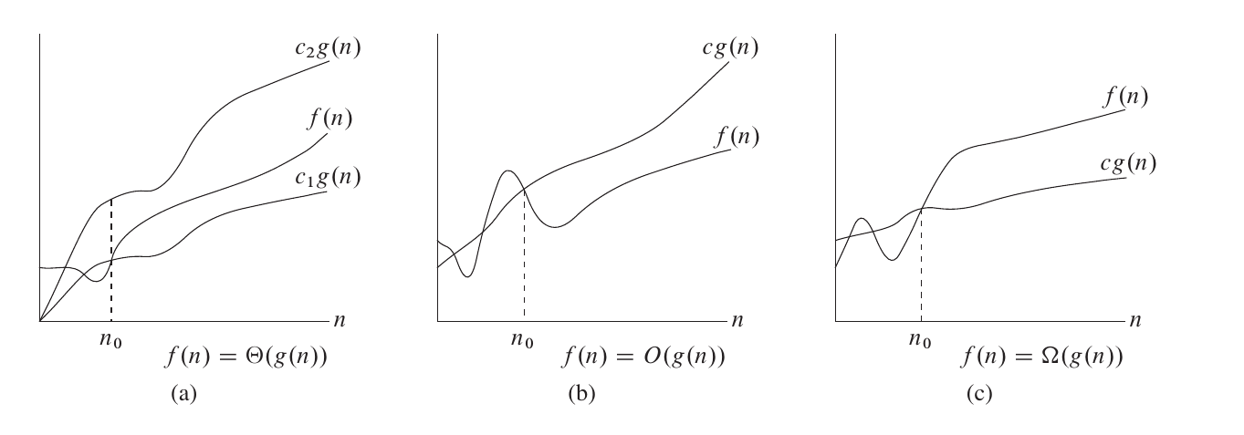
Θ-Notation
For functions and , we say $ f(n) = \Theta(g(n))$ if and only if .
In other words, it means by saying , we mean we can find two positive numbers and that satisfies .
For example, , .
Big O Notation
Θ-Notation both shows the upper and lower bound of a function. However, if we only know its asymptotical upper bound but not lower, we can use notation. We say if and only if .
It is more common to use big O notation while considering time complexity, as we are usually concerned with the upper bound of the program's time cost rather than the lower bound.
Note that the "upper" and "lower" bounds here are for the trend of the function, not for the algorithm, whose upper case refers to worst-case time complexity but not big O notation. Therefore, using Θ-notation is completely viable to represent worst-case time complexity, and it can even be said that Θ-notation is more accurate than big O notation. As for the main reason for using O notation more often, one is we sometimes can prove the upper bound, but not lower bound (this is usually the case for more complicated algorithm and analyzing its complexity), and the other reason is the character O is easier to input in a computer.
Ω-Notation
Similarly, we use Ω-Notation to describe the asymptotical lower bound of a function. We say if and only if .
o-Notation
If notation corresponds to the less-than-or-equal sign, then notation (or small o notation) correspond to the less-than sign. We say if and only if
ω-Notation
If notation is equivalent to the greater-than-or-equal sign, then notation(or small omega notation) is equivalent to the greater-than sign. That is, we say if and only if .
Common Properties
- . From the logarithm's change-of-base formula, we can conclude that, regardless of base, any logarithmic function has the same growth rate. Therefore, the base of an logarithm is often omitted in asymptotic time complexity.
Simple Examples of Calculating Time Complexity
for-expression
// C++ Version
int n, m;
std::cin >> n >> m;
for (int i = 0; i < n; ++i) {
  for (int j = 0; j < n; ++j) {
    for (int k = 0; k < m; ++k) {
      std::cout << "hello world\n";
    }
  }
}
# Python Version
n = int(input())
m = int(input())
for i in range(0, n):
for j in range(0, n):
for k in range(0, m):
print("hello world")The time complexity of the code above is if we consider the inputted value of and as the data size.
DFS
While performing depth-first search (article not translated) on a graph with points and edges, as each point and edges will be visited constant times, the complexity is .
Identifying Constants
When we are going to perform several operations, how to determine whether these several operations will impact time complexity? e.g.:
// C++ Version
const int N = 100000;
for (int i = 0; i < N; ++i) {
  std::cout << "hello world\n";
}
# Python Version
N = 100000
for i in range(0, N):
print("hello world")If the value of is not considered as data size of input, then time complexity of these blocks of code is .
When calculating time complexity, it is important to figure out which variables should be treated as the size of data size. All other variables not relating to input data size will be treated as constants and treated as (or constant time) when calculating time complexity.
Master Theorem
By using master theorem we can quickly calculate the time complexity of a recursive algorithm.
Assume we have a recurrence relation formula,
Then,
Amortized Complexity
Algorithms tend to modify data in memory, and multiple executions of an algorithm will have impact on each other by modifying data.
E.g., for the sorting-by-size operation in quicksort, the worst-case time complexity is seemed to be . But because of the divide-and-conquer process from quicksort, previous sorting operation constantly reduces the length of the array. Therefore, the actual overall complexity is , and the breakdowns over each sorting operation is .
The overall complexity of multiple operations divided by the number of operations is Amortized Complexity.
Potential Method of Amortized Analysis
Potential method of amortized analysis is a method for finding the upper bound of amortized complexity. The key to finding amortized complexity is to represent the impact to current operation from previous operation.
Definition of state: represents all data in specific moment. E.g., in quicksort, a "state" is an subscript interval needed to be sorted.
Definition of initial state: represents the state when no operation has been performed. E.g., in quicksort, an "initial state" is the whole array.
Assume is a function from state to number, and . Then we have the following inference:
Let be a sequence produced by performing times of operation from , and be the time cost of -th operation.
Let . Then the total time cost of times of operation is:
(It is obvious that positive and negative ones cancel)
And because we have
Therefore, if , then is an upper bound of amortized time complexity
Potential method have many tricks. Examples omitted here.
Space Complexity
Similarly, the growing trend of space cost with input sizes' growth can be measured by space complexity using similar methods mentioned above.
Calculate Complexity
The article mainly introduced complexity from the perspective of algorithm analysis. If interested you can visit Computational Complexity (not translated) for further reading.
buildLast update and/or translate time of this article,Check the history
editFound smelly bugs? Translation outdated? Wanna contribute with us? Edit this Page on Github
peopleContributor of this article linehk
translateTranslator of this article Visit the original article!
copyrightThe article is available under CC BY-SA 4.0 & SATA ; additional terms may apply.