Prefix Sum & Adjacent Difference
Last translate with upstream: be4fc67 on Mar 23, 2021
This article will briefly introduce prefix sum, and its opposite strategy, adjacent difference.
Prefix Sum
Prefix sum is an important kind of preprocessing, which can significantly reduce the time complexity of querying. It can be simply understood as "the sum of the first elements of an array".
C++ standard library has implemented the function of constructing prefix sum array std::partial_sum, defined in the header <numeric>.
Example
Example
You are given an array with positive integers. You are asked to construct a new array , where the -th element of new array represents the sum of the -th to -th elements of the original array .
Input:
5
1 2 3 4 5
Output:
1 3 6 10 15Solution
There are two approaches for this problem:
- Put the accumulative sum of array to array one by one.
- Iteration:
B[i] = B[i-1] + A[i], and specificallyB[0] = A[0]。
Example Solution Code
#include <iostream>
using namespace std;

int N, A[10000], B[10000];
int main() {
  cin >> N;
  for (int i = 0; i < N; i++) {
    cin >> A[i];
  }

  // First element of original array and prefix sum array are equivalent.
  B[0] = A[0];

  for (int i = 1; i < N; i++) {
    // i-th element of prefix sum array = sum of 0th to (i-1)-th elements of original array + i-th element of original array
    B[i] = B[i - 1] + A[i];
  }

  for (int i = 0; i < N; i++) {
    cout << B[i] << " ";
  }

  return 0;
}
2-Dimensional and Multi-Dimensional Prefix Sum
Approches for finding multi-dimensional prefix sum are mostly based on the inclusion-exclusion principle.
Example: Extending 1-dimensional prefix sum to 2-dimensional prefix sum.
For example, we have a matrix , which can be treated as a 2-dimension array
1 2 4 3
5 1 2 4
6 3 5 9
We define a matrix , where ,
1  3  7  10
6  9  15 22
12 18 29 45
The first problem is the process of finding by iteration: .
Because of the addition of and is duplicated with , here subtracted it.
The second problem is how to apply, e.g., calculate the sum of sub-matrixes .
Then we can easily conclude that based on similar idea.
Example
Luogu P1387
Given a matrix with only and . Your task is to find the largest square without in the matrix and print the length of its edge.
Example Solution Code
#include <algorithm>
#include <iostream>
using namespace std;
int a[103][103];
int b[103][103];  // Prefix sum array, which is equivalent to `sum[]` mentioned before.
int main() {
  int n, m;
  cin >> n >> m;

  for (int i = 1; i <= n; i++) {
    for (int j = 1; j <= m; j++) {
      cin >> a[i][j];
      b[i][j] =
          b[i][j - 1] + b[i - 1][j] - b[i - 1][j - 1] + a[i][j];  // Calculate the prefix sum.
    }
  }

  int ans = 1;

  int l = 2;
  while (l <= min(n, m)) {
    for (int i = l; i <= n; i++) {
      for (int j = l; j <= m; j++) {
        if (b[i][j] - b[i - l][j] - b[i][j - l] + b[i - l][j - l] == l * l) {
          ans = max(ans, l);
        }
      }
    }
    l++;
  }

  cout << ans << endl;
  return 0;
}
High-Dimensional Sum over Subsets Dynamic Programming
The method of calculating multi-dimensional prefix sum based on inclusion-exclusion principle has an advantage of simple form and no need to memorize specifically. But as the dimension increases, the algorithm would have high complexity. This section will introduce a method of calculating high-dimensional prefix sum based on dynamic programming.
Let to be a high-dimensional space with dimensions. We need to find the high-dimensional prefix sum of . Let represent all contribution to high-dimensional prefix sum of from all same node of -th dimension after . From the definition we know that and .
The iteration is , where is all node that smaller than in -th dimension, where is the size of high-dimensional space .
Here is an example of implementation in pseudocode:
    for state
      sum[state] = f[state];
    for(i = 0;i <= D;i += 1)
      for state (in lexicographic order)
        sum[state] += sum[state'];
Prefix Sum on Tree
Let represent the sum of weight from node to root node. Then:
- If weight is on nodes: Sum in path is .
- If weight is on edges: Sum in path is .
About how to calculate please refer to Lowest Common Ancestor.
Adjacent Difference
Adjacent difference is a strategy opposite to prefix sum, which can be treated as an inverse operation to sum.
The definition is let .
Simple properties:
- is prefix sum of , i.e., .
- Calculate prefix sum of :
This can maintain the time complexity of query an element after adding a number multiply to an interval, or multiply query a element. Note that modifying operations should be former to querying operations.
Example
For example, adding to every element in is
where ,.
And perform prefix sum once in the end.
C++ standard library has the implementation of constructing an adjacent difference array std::adjacent_difference,defined in header file <numeric>.
Adjacent Difference on Tree
The phrase, adjacent difference on tree, can be understood as performing adjacent difference on some path of tree, where "path" can be comprehended similar to the interval in one-dimensional array. Adjacent difference on tree can be used when, for example, operating intensively on some paths, and querying the value of some edge or node after operating.
In competitive programming, related problems are sometimes solved in accompany with tree and LCA. In further, adjacent difference on tree can be divided into difference on node and difference on edge with slight difference in implementation.
Difference on Node
Example: Access some paths in a domain tree . Find out how many times the nodes in a path have been accessed.
For an access to we need to find the LCA of and , and accessing all nodes in the path by adding 1 on their weight. Because there are enormous nodes needed to be accessed, we cannot afford the time cost if we adopt a DFS algorithm to access every node. Therefore here performs adjacent difference.
Where represents the parent node of $lca#, and is the adjacent difference array of node weight array ,
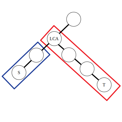
In the illustration, we can acknowledge that the former two formulas operate the path tagged by blue rectangle, and latter two operate the path tagged by red rectangle. Why not name the immediate child node to the left side of ad . In this case we have ,. We can conclude that the operations of difference on edge is similar to difference on one-dimensional array.
Difference on Edge
We need to adopt the strategy of adjacent difference on edge when accessing edges in some path. We use the following formulas:
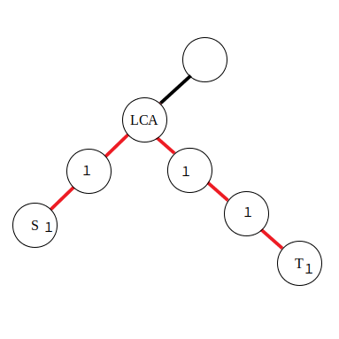
Because of the difficulty of calculating difference on edges, for handy operation, we move the value which is supposed to accumulate to red edge down to nearby node. As for the formulas, it is not hard to derive with knowledge of difference on nodes that performs difference to two intervals.
Example problem
USACO 2015 December Contest, Platinum Problem 1. Max Flow
Farmer John has installed a new system of pipes to transport milk between the N stalls in his barn , conveniently numbered . Each pipe connects a pair of stalls, and all stalls are connected to each-other via paths of pipes.
FJ is pumping milk between pairs of stalls . For the ith such pair, you are told two stalls and , endpoints of a path along which milk is being pumped at a unit rate. FJ is concerned that some stalls might end up overwhelmed with all the milk being pumped through them, since a stall can serve as a waypoint along many of the paths along which milk is being pumped. Please help him determine the maximum amount of milk being pumped through any stall. If milk is being pumped along a path from to , then it counts as being pumped through the endpoint stalls and , as well as through every stall along the path between them.
Analysis of Problem
Because it is needed to count how many times has been every node accessed, by using the method of adjacent difference on tree to add on every node on every path, we can quickly get the number of accessing of nodes. Here uses binary lifting to calculate LCA. In the end by using DFS to traverse the whole tree, we can find the answer by calculate the sum of adjacent difference array when backtracking.
Example Solution Code
#include <bits/stdc++.h>

using namespace std;
#define maxn 50010

struct node {
  int to, next;
} edge[maxn << 1];

int fa[maxn][30], head[maxn << 1];
int power[maxn];
int depth[maxn], lg[maxn];
int n, k, ans = 0, tot = 0;

void add(int x, int y) {
  edge[++tot].to = y;
  edge[tot].next = head[x];
  head[x] = tot;
}

void dfs(int now, int father) {
  fa[now][0] = father;
  depth[now] = depth[father] + 1;
  for (int i = 1; i <= lg[depth[now]]; ++i)
    fa[now][i] = fa[fa[now][i - 1]][i - 1];
  for (int i = head[now]; i; i = edge[i].next)
    if (edge[i].to != father) dfs(edge[i].to, now);
}

int lca(int x, int y) {
  if (depth[x] < depth[y]) swap(x, y);
  while (depth[x] > depth[y]) x = fa[x][lg[depth[x] - depth[y]] - 1];
  if (x == y) return x;
  for (int k = lg[depth[x]] - 1; k >= 0; k--) {
    if (fa[x][k] != fa[y][k]) x = fa[x][k], y = fa[y][k];
  }
  return fa[x][0];
}

// Calculate the maximum amount of milk being pumped, and add the weight of sub-tree when backtracking.
void get_ans(int u, int father) {
  for (int i = head[u]; i; i = edge[i].next) {
    int to = edge[i].to;
    if (to == father) continue;
    get_ans(to, u);
    power[u] += power[to];
  }
  ans = max(ans, power[u]);
}

int main() {
  scanf("%d %d", &n, &k);
  int x, y;
  for (int i = 1; i <= n; i++) {
    lg[i] = lg[i - 1] + (1 << lg[i - 1] == i);
  }
  for (int i = 1; i <= n - 1; i++) {
    scanf("%d %d", &x, &y);
    add(x, y);
    add(y, x);
  }
  dfs(1, 0);
  int s, t;
  for (int i = 1; i <= k; i++) {
    scanf("%d %d", &s, &t);
    int ancestor = lca(s, t);
    // Adjacent difference on tree
    power[s]++;
    power[t]++;
    power[ancestor]--;
    power[fa[ancestor][0]]--;
  }
  get_ans(1, 0);
  printf("%d\n", ans);
  return 0;
}
Exercises
Prefix Sum:
- (Chinese) Luogu U53525 Prefix Sum
- (Chinese) Luogu U69096 Reverse Prefix Sum
- 6th JOI Final: The Largest Sum Judge is here.
- USACO 2016 January Contest, Silver Problem 2. Subsequences Summing to Sevens
2-Dimensional and Multi-Dimensional Prefix Sum:
- HDU 6514 Monitor
- (Chinese) Luogu P1387 Largest Square
- (Chinese) HNOI2003 Laser Bomb
Prefix Sum on Tree
- (Chinese) LOJ 10134. Dis
- (Chinese) LOJ 2491. 求和
Adjacent Difference:
- (Chinese) LOJ 132. Fenwick Tree III
- (Chinese) Luogu P3397 Carpet
- (Chinese) Luogu P4552 「Poetize6」IncDec Sequence
Adjacent Difference on Tree:
- USACO 2015 December Contest, Platinum Problem 1. Max Flow
- (Chinese) JLOI2014 Squirrel's New Home
- (Chinese) NOIP2015 Transportation Planning
- (Chinese) NOIP2016 Running Everyday
buildLast update and/or translate time of this article,Check the history
editFound smelly bugs? Translation outdated? Wanna contribute with us? Edit this Page on Github
peopleContributor of this article OI-wiki
translateTranslator of this article Visit the original article!
copyrightThe article is available under CC BY-SA 4.0 & SATA ; additional terms may apply.